Examples: Analysis of Real Jumps
This page analyses several jumps in which people have been injured on. The jumps have been measured by the package authors over the years. The intention is to show the utility of the software for analyzing arbitrary jump shapes and to highlight the large equivalent fall heights of these jump constructions. The jumps are idenified by location and the year it was measured.
Import packages needed on this page:
import numpy as np
import matplotlib.pyplot as plt
from skijumpdesign import Skier, Surface
from skijumpdesign.functions import (
    make_jump, plot_efh, cartesian_from_measurements)
Selection of an Equivalent Fall Height
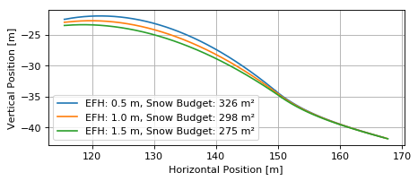
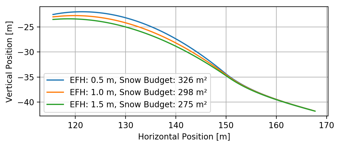
Beginner ski slopes range from 6% to 25% grade (3 to 14 degrees) and intermediate ski slopes range from 25% to 40% (14 to 22 degrees) [1]. Terrain parks are typically built on steeper beginner slopes or shallow intermediate slopes, thus a parent slope grade of 25% (14 degrees) is a reasonable choice to compare the snow budgets of different jumps designed with equivalent fall heights. The following plot shows how the snow budget increases as EFH decreases.
parent_slope_grade = 0.25  # percent grade
parent_slope_angle = -np.rad2deg(np.arctan(parent_slope_grade))  # degrees
approach_length = 100.0  # meters
takeoff_angle = 20.0  # degrees

fig, ax = plt.subplots(1, 1)

for efh, color in zip((0.5, 1.0, 1.5), ('C0', 'C1', 'C2')):
   jump = make_jump(parent_slope_angle, 0.0, approach_length,
                    takeoff_angle, efh)
   snow_budget = jump[-1]['Snow Budget']
   for i, surf in enumerate(jump[3:-2]):
      if i % 2 == 1:
         lab = 'EFH: {:1.1f} m, Snow Budget: {:1.0f} m²'.format(efh, snow_budget)
      else:
         lab = None
      surf.plot(ax=ax, color=color, label=lab)

ax.set_xlabel('Horizontal Position [m]')
ax.set_ylabel('Vertical Position [m]')
ax.set_aspect('equal')
ax.legend()
ax.grid()
(Source code, png, hires.png, pdf)

An equivalent fall height of 1.5 m will, on average, cause knee collapse in an adult [2]. This is a sensible absolute maximal boundary for equivalent fall height in constructed jumps. An equivalent fall height of 0.5 m is a fairly benign height, similar to falling from two or three stair steps. A height of 1 m is a good compromise between these two numbers that has a reasonable snow budget with moderate height. The following jumps will compared to jumps designed with a 1 m equivalent fall height for this reason.
| [1] | https://en.wikipedia.org/wiki/Piste |
| [2] | A. E. Minetti, “Using leg muscles as shock absorbers: theoretical predictions and experimental results of drop landing performance,” Ergonomics, vol. 41, no. 12, pp. 1771–1791, Dec. 1998, doi: 10.1080/001401398185965. |
Design Speed
The “design speed” for a constant equivalent fall height jump is defined in [3] as:
The maximum takeoff velocity (resulting from the highest start point and minimum snow friction \(\mu\) and air drag \(\eta\)) is called the design speed.
It is the maximum expected takeoff speed of a skier or snowboarder, which is a function of the inrun length, slope, friction coefficient, and air drag. The designed jumps ensure a constant equivalent fall height up to this design speed.
| [3] | Levy, Dean, Mont Hubbard, James A. McNeil, and Andrew Swedberg. “A Design Rationale for Safer Terrain Park Jumps That Limit Equivalent Fall Height.” Sports Engineering 18, no. 4 (December 2015): 227–39. https://doi.org/10.1007/s12283-015-0182-6. |
California 2002
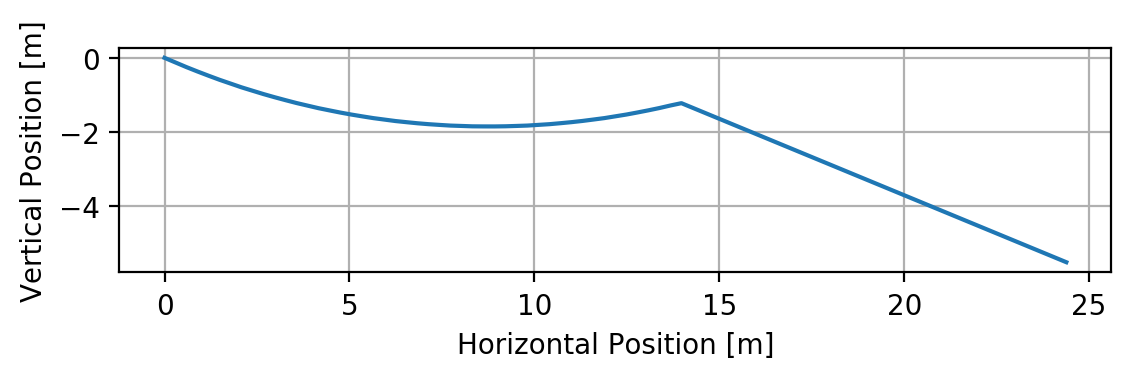
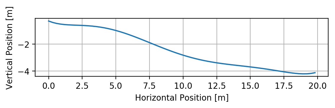
The california-2002-surface.csv file contains the horizontal (x)
and vertical (y) coordinates of a jump measured at a ski resort in California,
USA in 2002. The comma separated value file can be loaded with
numpy.loadtxt() and used to create a
Surface. The
plot() method is used to quickly
visualize the measured landing surface. The takeoff location is situated at
(x=0 m, y=0 m).
landing_surface_data = np.loadtxt('california-2002-surface.csv',
                                  delimiter=',',  # comma separated
                                  skiprows=1)  # skip the header row

landing_surface = Surface(landing_surface_data[:, 0],  # x values in meters
                          landing_surface_data[:, 1])  # y values in meters

ax = landing_surface.plot()
(Source code, png, hires.png, pdf)

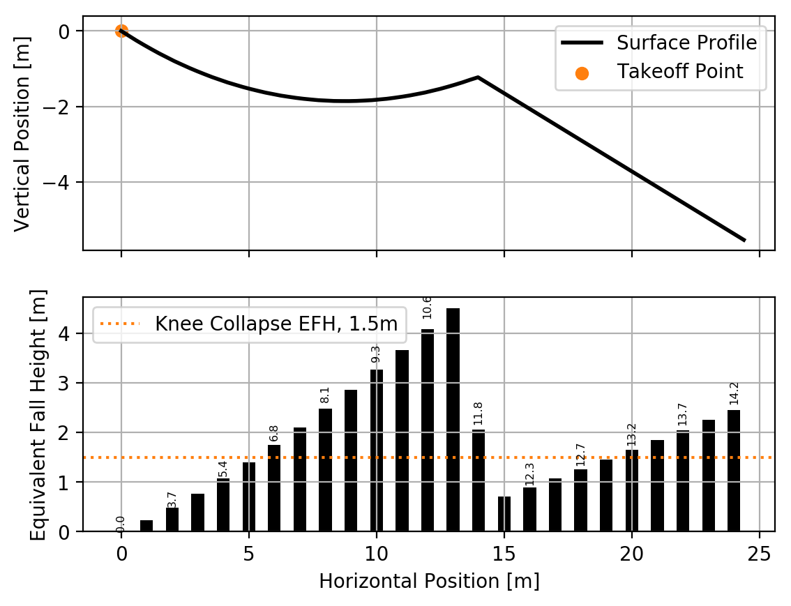
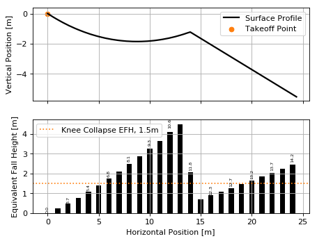
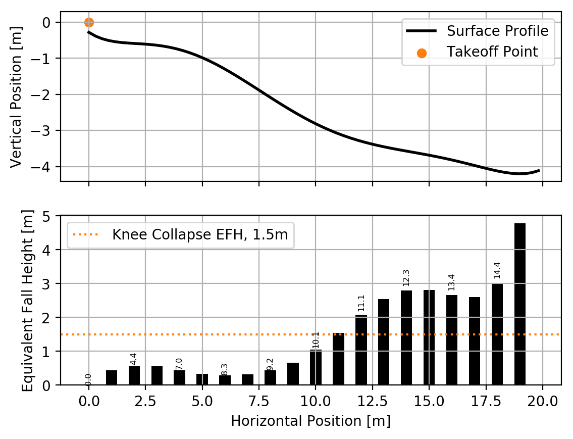
The takeoff angle of this jump was measured as 13 degrees. Using this angle the equivalent fall height can be visualized across the landing surface.
takeoff_angle = 30.0  # degrees
takeoff_point = (0.0, 0.0)  # meters

skier = Skier()

plot_efh(landing_surface, takeoff_angle, takeoff_point,
         skier=skier, increment=1.0)
(Source code, png, hires.png, pdf)
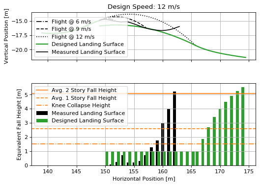
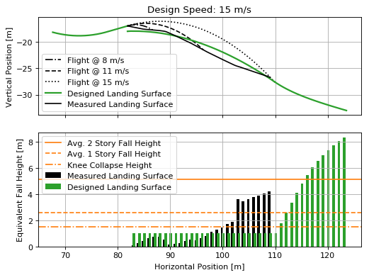
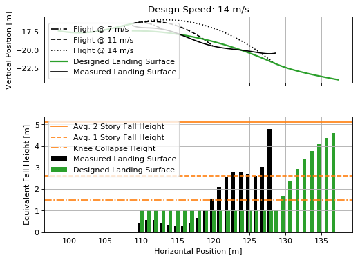
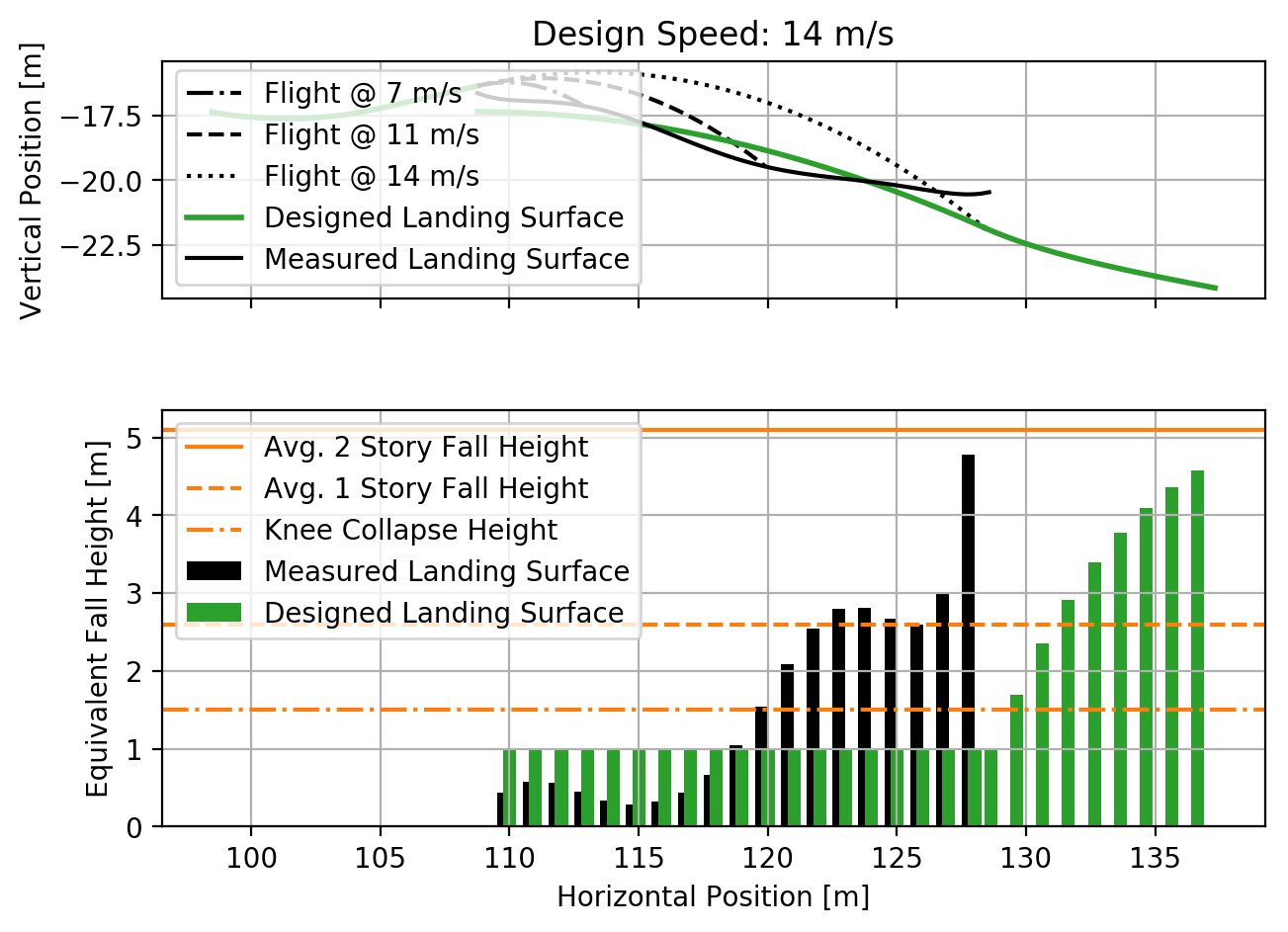
The actual jump can be compared to a jump designed with a constant equivalent fall height. The figure below shows such a comparison.
def compare_measured_to_designed(measured_surface, equiv_fall_height,
                                 parent_slope_angle, approach_length,
                                 takeoff_angle, skier):

    # NOTE : A different Skier() object is used internally in make_jump()
    slope, approach, takeoff, landing, landing_trans, flight, outputs = \
        make_jump(parent_slope_angle, 0.0, approach_length, takeoff_angle,
                  equiv_fall_height)

    measured_surface.shift_coordinates(takeoff.end[0], takeoff.end[1])

    design_speed = flight.speed[0]
    low_speed = 1/2*design_speed
    med_speed = 3/4*design_speed

    vel_vec = np.array([np.cos(np.deg2rad(takeoff_angle)),
                        np.sin(np.deg2rad(takeoff_angle))])

    flight_low = skier.fly_to(measured_surface, init_pos=takeoff.end,
                              init_vel=tuple(low_speed*vel_vec))
    flight_med = skier.fly_to(measured_surface, init_pos=takeoff.end,
                              init_vel=tuple(med_speed*vel_vec))

    fig, (prof_ax, efh_ax) = plt.subplots(2, 1, sharex=True,
                                          constrained_layout=True)

    increment = 1.0

    dist, efh, _ = measured_surface.calculate_efh(np.deg2rad(takeoff_angle),
                                                  takeoff.end, skier, increment)

    efh_ax.bar(dist, efh, color='black', align='center', width=increment/2,
               label="Measured Landing Surface")

    dist, efh, _ = landing.calculate_efh(np.deg2rad(takeoff_angle),
                                         takeoff.end, skier, increment)

    efh_ax.bar(dist, efh, color='C2', align='edge', width=increment/2,
               label="Designed Landing Surface")

    dist, efh, _ = landing_trans.calculate_efh(np.deg2rad(takeoff_angle),
                                               takeoff.end, skier, increment)

    efh_ax.bar(dist, efh, color='C2', align='edge', width=increment/2,
               label=None)

    efh_ax.axhline(5.1, color='C1', label='Avg. 2 Story Fall Height')
    efh_ax.axhline(2.6, color='C1', linestyle='dashed',
                   label='Avg. 1 Story Fall Height')
    efh_ax.axhline(1.5, color='C1', linestyle='dashdot',
                   label='Knee Collapse Height')

    prof_ax = takeoff.plot(ax=prof_ax, linewidth=2, color='C2', label=None)

    prof_ax = flight_low.plot(ax=prof_ax, color='black', linestyle='dashdot',
                              label='Flight @ {:1.0f} m/s'.format(low_speed))
    prof_ax = flight_med.plot(ax=prof_ax, color='black', linestyle='dashed',
                              label='Flight @ {:1.0f} m/s'.format(med_speed))
    prof_ax = flight.plot(ax=prof_ax, color='black', linestyle='dotted',
                          label='Flight @ {:1.0f} m/s'.format(design_speed))

    prof_ax = landing.plot(ax=prof_ax, color='C2', linewidth=2, label=None)
    prof_ax = landing_trans.plot(ax=prof_ax, color='C2', linewidth=2,
                                 label='Designed Landing Surface')

    prof_ax = measured_surface.plot(ax=prof_ax, color='black',
                                    label="Measured Landing Surface")

    prof_ax.set_title('Design Speed: {:1.0f} m/s'.format(design_speed))

    prof_ax.set_ylabel('Vertical Position [m]')
    efh_ax.set_ylabel('Equivalent Fall Height [m]')
    efh_ax.set_xlabel('Horizontal Position [m]')

    efh_ax.grid()
    prof_ax.grid()
    efh_ax.legend(loc='upper left')
    prof_ax.legend(loc='lower left')

    return prof_ax, efh_ax
fall_height = 1.0  # meters
slope_angle = -8.0  # degrees
approach_length = 180.0  # meters

compare_measured_to_designed(landing_surface, fall_height, slope_angle,
                             approach_length, takeoff_angle, skier)
(Source code, png, hires.png, pdf)
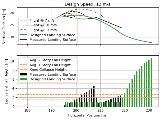
The average story heights are estimated from [4].
| [4] | N. L. Vish, “Pediatric window falls: not just a problem for children in high rises,” Injury Prevention, vol. 11, no. 5, pp. 300–303, Oct. 2005, doi: 10.1136/ip.2005.008664. |
Washington 2004
The washington-2004-surface.csv file contains the horizontal (x)
and vertical (y) coordinates of a jump measured at a Washington, USA ski resort
in 2004. The comma separated value file can be loaded with numpy.loadtxt()
and used to create a Surface. The
plot() method is used to quickly
visualize the measured landing surface. The takeoff location is situated at
(x=0 m, y=0 m).
landing_surface_data = np.loadtxt('washington-2004-surface.csv',
                                  delimiter=',',  # comma separated
                                  skiprows=1)  # skip the header row

landing_surface = Surface(landing_surface_data[:, 0],  # x values in meters
                          landing_surface_data[:, 1])  # y values in meters

ax = landing_surface.plot()
(Source code, png, hires.png, pdf)
The takeoff angle of this jump was measured as 25 degrees. Using this angle the equivalent fall height can be visualized across the landing surface.
takeoff_angle = 25.0  # degrees
takeoff_point = (0.0, 0.0)  # meters

skier = Skier()

plot_efh(landing_surface, takeoff_angle, takeoff_point,
         skier=skier, increment=1.0)
(Source code, png, hires.png, pdf)
For high takeoff speeds, this jump has very large equivalent fall heights (3 m to 13 m).
The actual jump can be compared to a jump designed with a constant equivalent fall height. The figure below shows such a comparison. Note that the first 15 meters or so of the surface is reasonable, but if a jumper lands beyond 15 m they will be subjected to dangerous impact velocities.
fall_height = 1.0  # meters
slope_angle = -10.0  # degrees
approach_length = 220.0  # meters

compare_measured_to_designed(landing_surface, fall_height, slope_angle,
                             approach_length, takeoff_angle, skier)
(Source code, png, hires.png, pdf)

Utah 2010
The utah-2010-surface.csv file contains the horizontal (x) and
vertical (y) coordinates of a jump measured at a Utah, USA ski resort in
February 2010. The comma separated value file can be loaded with
numpy.loadtxt() and used to create a
Surface. The
plot() method is used to quickly
visualize the measured landing surface. The takeoff location is situated at
(x=0 m, y=0 m).
landing_surface_data = np.loadtxt('utah-2010-surface.csv',
                                  delimiter=',',  # comma separated
                                  skiprows=1)  # skip the header row

landing_surface = Surface(landing_surface_data[:, 0],  # x values in meters
                          landing_surface_data[:, 1])  # y values in meters

ax = landing_surface.plot()
(Source code, png, hires.png, pdf)
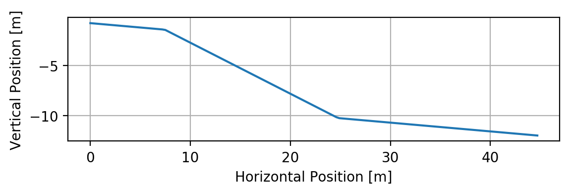
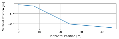
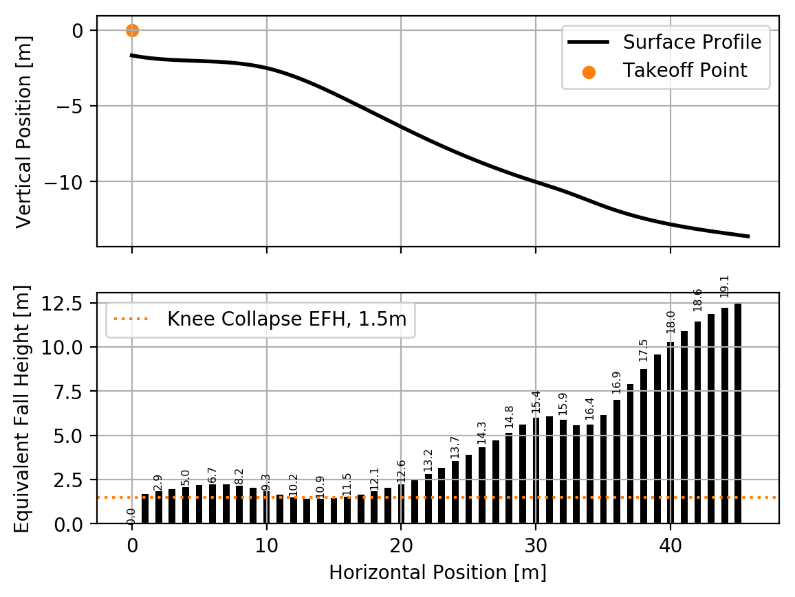
The takeoff angle of this jump was measured as 23 degrees. Using this angle the equivalent fall height can be visualized across the landing surface.
takeoff_angle = 23.0  # degrees
takeoff_point = (0.0, 0.0)  # meters

skier = Skier()

plot_efh(landing_surface, takeoff_angle, takeoff_point,
         skier=skier, increment=1.0)
(Source code, png, hires.png, pdf)
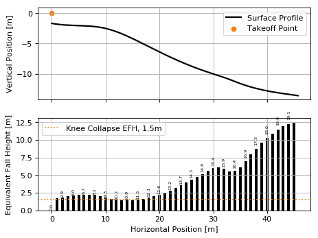
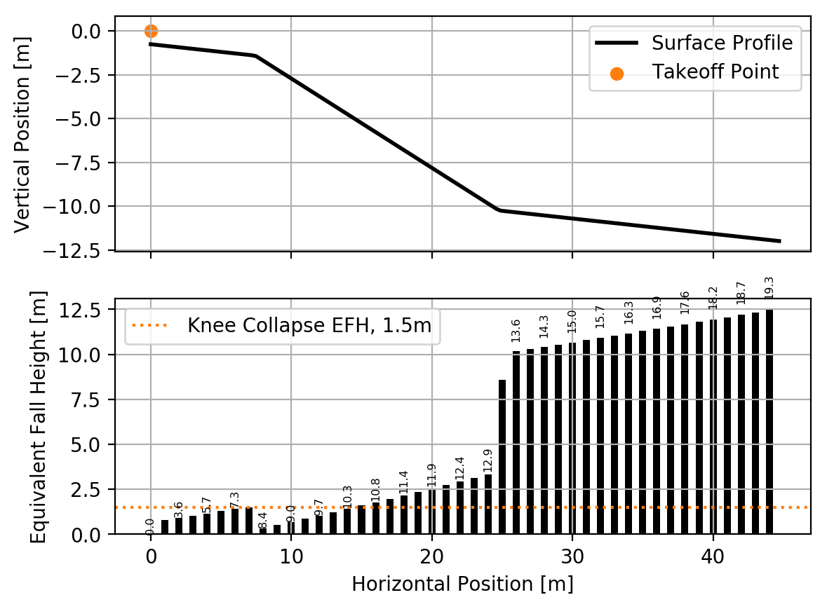
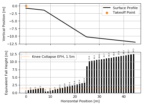
For high takeoff speeds, this jump has very large equivalent fall heights (5 m to 10 m). And no mater the takeoff speed, the equivalent fall height is greater than or equal to the 1.5 m threshold for knee collapse.
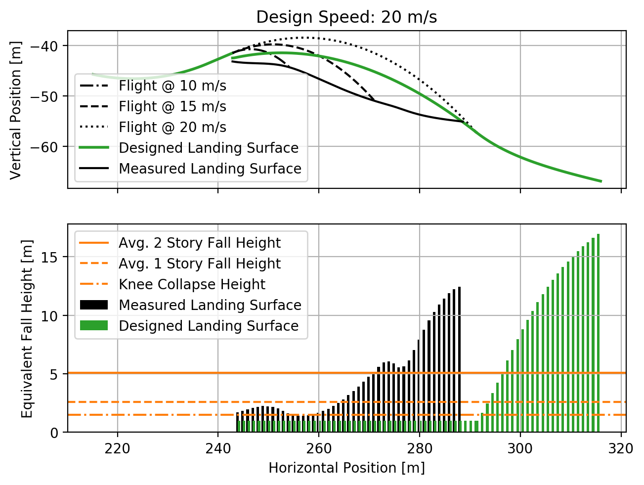
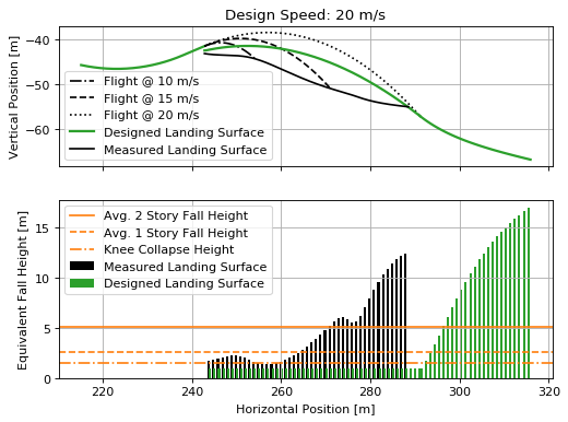
The measured jump can be compared to a jump designed to ensure a constant equivalent fall height of 1.5 m at any takeoff speed. The figure below shows such a comparison. Note that the first 15 meters or so of the surface is reasonable, but if a jumper lands beyond 15 m they will be subjected to dangerous impact speeds.
fall_height = 1.0  # meters
slope_angle = -12.0  # degrees
approach_length = 220.0  # meters

compare_measured_to_designed(landing_surface, fall_height, slope_angle,
                             approach_length, takeoff_angle, skier)
(Source code, png, hires.png, pdf)
Colorado 2009
The colorado-2009-surface.csv file contains the horizontal (x) and
vertical (y) coordinates of a jump measured by professional surveyors at a
Colorado, USA ski resort in March 2009. The comma separated value file can be
loaded with numpy.loadtxt() and used to create a
Surface. The
plot() method is used to quickly
visualize the measured landing surface. The takeoff location is situated at
(x=0 m, y=0 m).
landing_surface_data = np.loadtxt('colorado-2009-surface.csv',
                                  delimiter=',',  # comma separated
                                  skiprows=1)  # skip the header row

landing_surface = Surface(landing_surface_data[:, 0],  # x values in meters
                          landing_surface_data[:, 1])  # y values in meters

ax = landing_surface.plot()
(Source code, png, hires.png, pdf)

The takeoff angle of this jump was measured as 16 degrees. Using this angle the equivalent fall height can be visualized across the landing surface.
takeoff_angle = 16.0  # degrees
takeoff_point = (0.0, 0.0)  # meters

skier = Skier()

plot_efh(landing_surface, takeoff_angle, takeoff_point,
         skier=skier, increment=1.0)
(Source code, png, hires.png, pdf)
The actual jump can be compared to a jump designed with a constant equivalent fall height. The figure below shows such a comparison.
fall_height = 1.0  # meters
slope_angle = -15.0  # degrees
approach_length = 70.0  # meters

compare_measured_to_designed(landing_surface, fall_height, slope_angle,
                             approach_length, takeoff_angle, skier)
(Source code, png, hires.png, pdf)

Wisconsin 2015
The wisconsin-2015-surface.csv file contains the horizontal (x) and
vertical (y) coordinates of a jump measured at a Wisconsin, USA ski resort in
2015. The comma separated value file can be loaded with numpy.loadtxt() and
used to create a Surface. The
plot() method is used to quickly
visualize the measured landing surface. The takeoff location is situated at
(x=0 m, y=0 m).
landing_surface_data = np.loadtxt('wisconsin-2015-surface.csv',
                                  delimiter=',',  # comma separated
                                  skiprows=1)  # skip the header row

landing_surface = Surface(landing_surface_data[:, 0],  # x values in meters
                          landing_surface_data[:, 1])  # y values in meters

ax = landing_surface.plot()
(Source code, png, hires.png, pdf)
The takeoff angle of this jump was measured as 13 degrees. Using this angle the equivalent fall height can be visualized across the landing surface.
takeoff_angle = 13.0  # degrees
takeoff_point = (0.0, 0.0)  # meters

skier = Skier()

plot_efh(landing_surface, takeoff_angle, takeoff_point,
         skier=skier, increment=1.0)
(Source code, png, hires.png, pdf)

The actual jump can be compared to a jump designed with a constant equivalent fall height. The figure below shows such a comparison.
fall_height = 1.0  # meters
slope_angle = -10.0  # degrees
approach_length = 100.0  # meters

compare_measured_to_designed(landing_surface, fall_height, slope_angle,
                             approach_length, takeoff_angle, skier)
(Source code, png, hires.png, pdf)

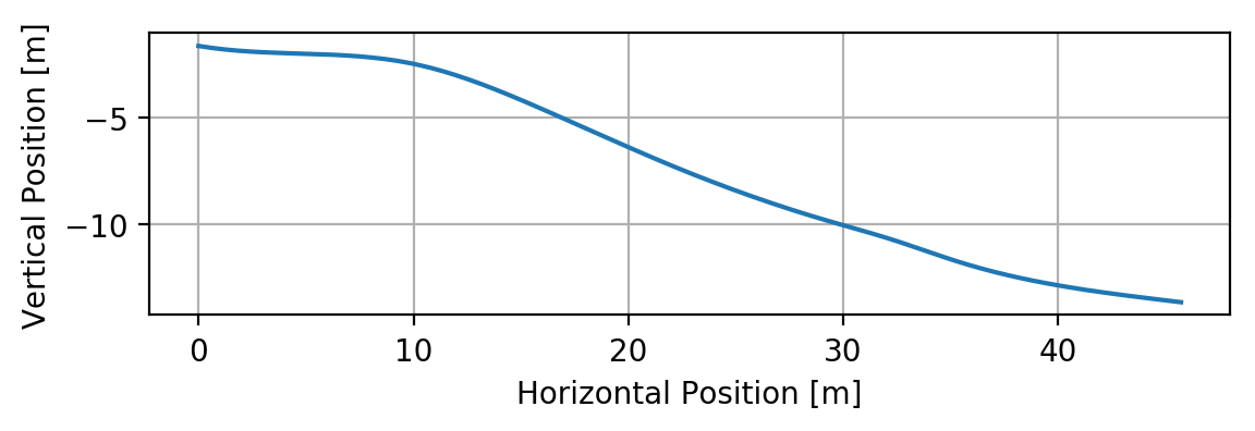
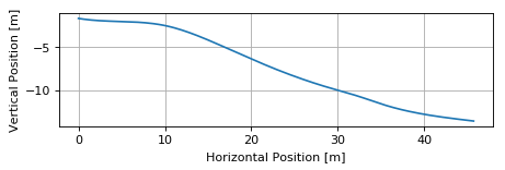
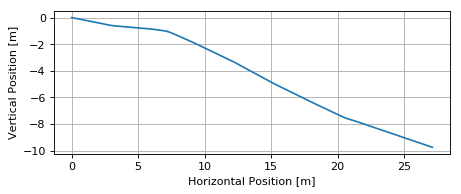
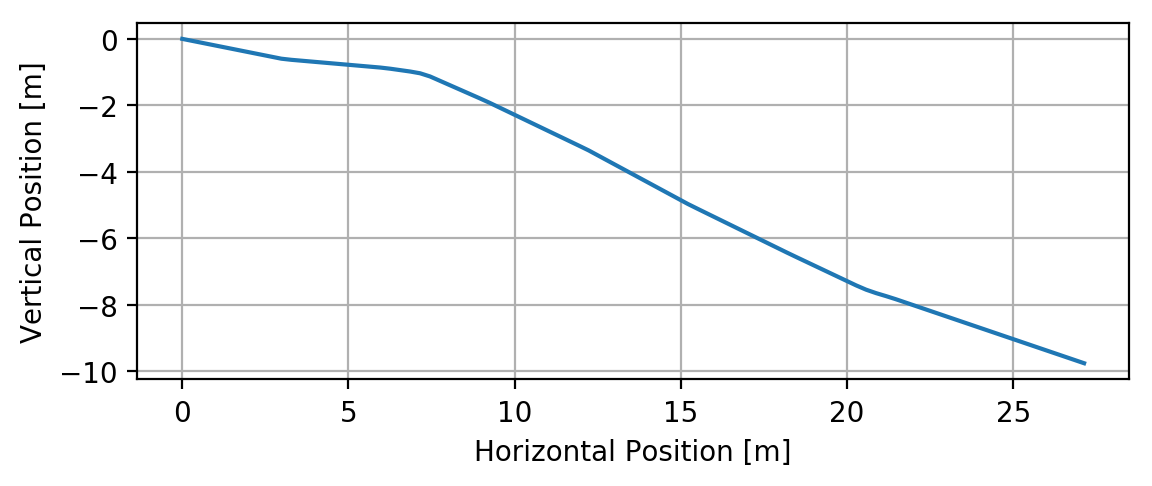
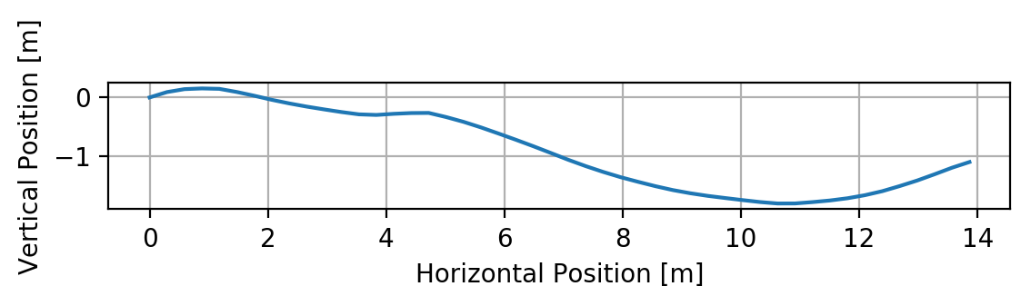
Sydney 2020
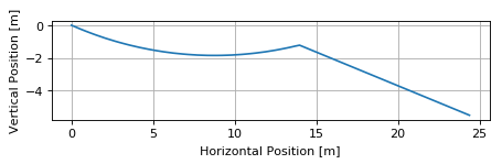
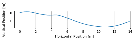
The sydney-measurements-2020.csv file contains the distance along
the jump surface and absolute angle measurements (different measures than all
above files) of a single-track dirt mountain bike jump measured near Sydney,
Australia in 2020. The comma separated value file can be loaded with
numpy.loadtxt(). These measurements require conversion to the Cartesian
coordinates for constructing the surface using
cartesian_from_measurements(). After conversion
the data can be used to create a Surface. The
plot() method is used to quickly
visualize the measured landing surface. The takeoff location is situated at the
first measurement point.
surface_measurement_data = np.loadtxt('sydney-measurements-2020.csv',
                                      delimiter=',',  # comma separated
                                      skiprows=1)  # skip the header row

x, y, takeoff_point, takeoff_angle = cartesian_from_measurements(
    surface_measurement_data[:, 0],  # distance along surface in meters
    np.deg2rad(surface_measurement_data[:, 1]))  # absolute angle deg -> rad

landing_surface = Surface(x,  # x values in meters
                          y)  # y values in meters

ax = landing_surface.plot()
(Source code, png, hires.png, pdf)

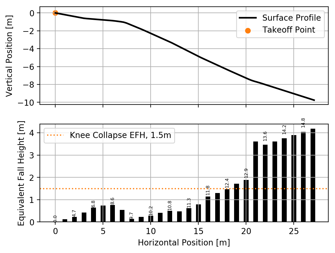
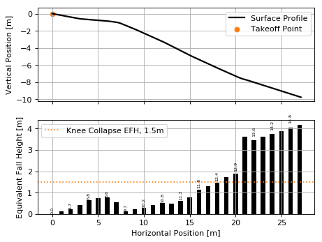
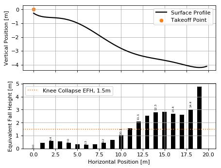
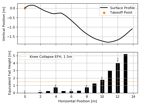
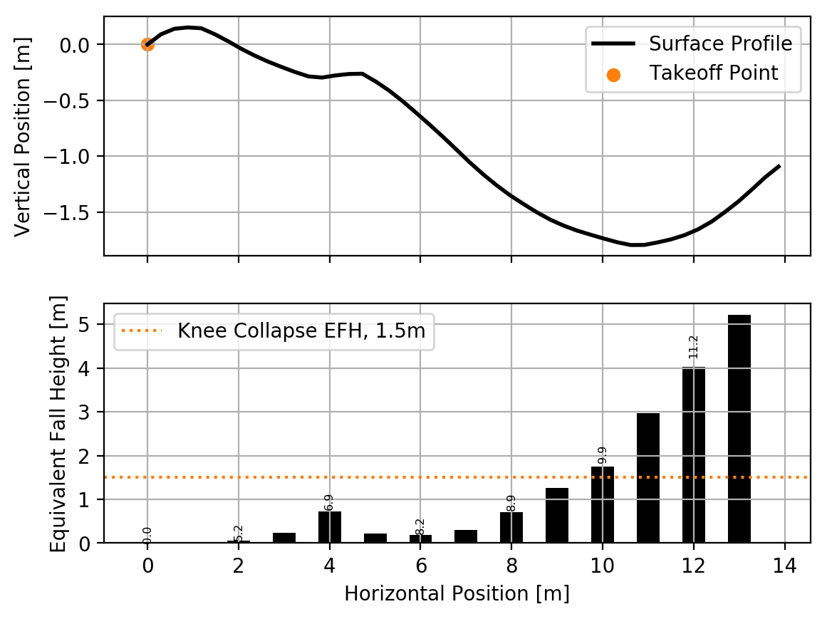
The takeoff angle is taken from the angle measurements. Using this angle the equivalent fall height can be visualized across the landing surface.
skier = Skier()

plot_efh(landing_surface, np.rad2deg(takeoff_angle), takeoff_point,
         skier=skier, increment=1.0)
(Source code, png, hires.png, pdf)

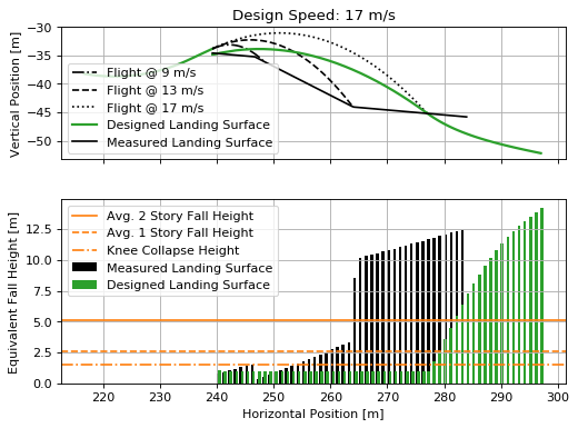
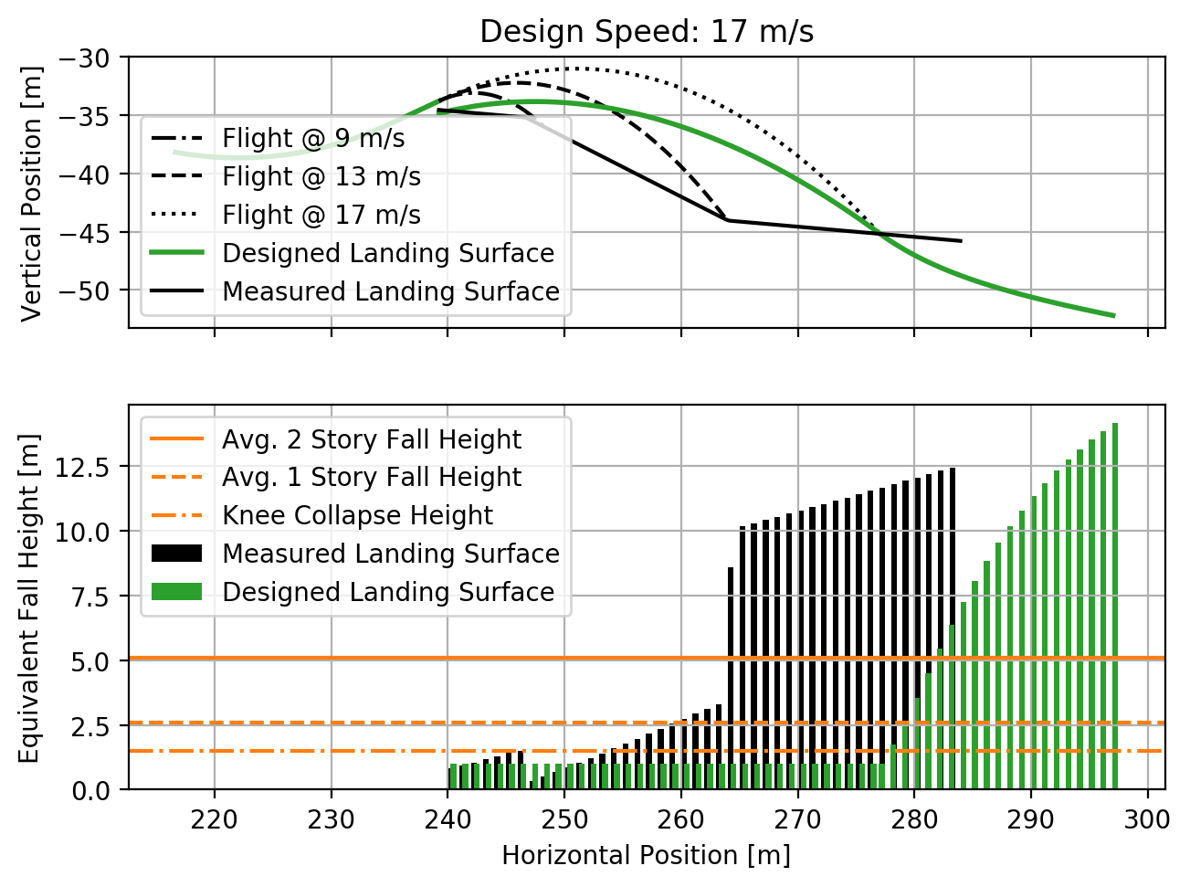
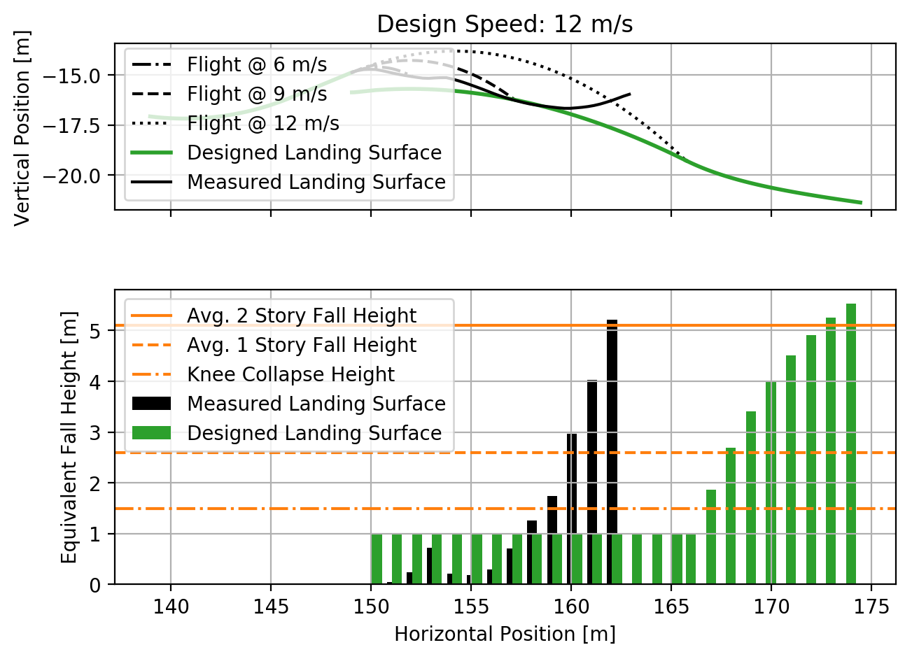
The actual jump can be compared to a jump designed with a constant equivalent fall height. The figure below shows such a comparison.
fall_height = 1.0  # meters
slope_angle = -7.0  # degrees
approach_length = 140.0  # meters

compare_measured_to_designed(landing_surface, fall_height, slope_angle,
                             approach_length, np.rad2deg(takeoff_angle), skier)
(Source code, png, hires.png, pdf)